Analyze dataset
2021-12-10
About
Description
This section is by far the busiest of the four that precede the article. In this section bar charts and maps are created for each of the groups of terms, and chi-squared tests are conducted on each to determine the nature of each term’s distribution. These three features serve as the foundation for all prose analysis about the data.
Usage
After loading in the necessary packages, code should be run for each updated CSV creating a bar chart, a contingency table, and a map, as well as code conducting a chi-square test and further analysis on the results of this test. The chunks necessary for these actions are labeled below, and the only thing that needs to be changed out is the name of the updated CSV.
Setup
# Script-specific options or packages
library(tidyverse)     # data manipulation
library(knitr)         # table output

library(janitor)
library(patchwork)
library(broom)
library(effectsize)
Run
plurals <- read_csv(file = "../data/original/twitter/plurals.csv")## Warning: One or more parsing issues, see `problems()` for detailssales <- read_csv(file = "../data/original/twitter/sales.csv")## Warning: One or more parsing issues, see `problems()` for detailsshoes <- read_csv(file = "../data/original/twitter/shoes.csv")## Warning: One or more parsing issues, see `problems()` for detailstonix <- read_csv(file = "../data/original/twitter/tonix.csv")## Warning: One or more parsing issues, see `problems()` for detailsroads <- read_csv(file = "../data/original/twitter/roads.csv")## Warning: One or more parsing issues, see `problems()` for detailsupdated_plurals <- read_csv(file = "../data/derived/updated_plurals.csv")
updated_sales <- read_csv(file = "../data/derived/updated_sales.csv")
updated_shoes <- read_csv(file = "../data/derived/updated_shoes.csv")
updated_tonix <- read_csv(file = "../data/derived/updated_tonix.csv")## Warning: One or more parsing issues, see `problems()` for detailsupdated_roads <- read_csv(file = "../data/derived/updated_roads.csv")## Warning: One or more parsing issues, see `problems()` for detailsSecond Person Plurals
updated_plurals %>%
  tabyl(search_term, census_region) %>% # cross-tabulate
  adorn_totals(c("row", "col")) %>% # provide row and column totals
  adorn_percentages("col") %>% # add percentages to the columns
  adorn_pct_formatting(rounding = "half up", digits = 0) %>% # round the digits
  adorn_ns() %>% # add observation number
  adorn_title("combined") %>% # add a header title
  kable(booktabs = TRUE, # pretty table
caption = "Contingency table for `search_term` and `census_region`.") # caption| search_term/census_region | Midwest | Northeast | South | West | Total |
|---|---|---|---|---|---|
| “you guys” | 43% (9) | 44% (7) | 20% (13) | 36% (10) | 30% (39) |
| y’all | 24% (5) | 25% (4) | 33% (21) | 36% (10) | 31% (40) |
| yall | 33% (7) | 31% (5) | 47% (30) | 29% (8) | 39% (50) |
| Total | 100% (21) | 100% (16) | 100% (64) | 100% (28) | 100% (129) |
p1 <-
  updated_plurals %>% # dataset
  ggplot(aes(x = census_region, fill = search_term)) + # mappings
  geom_bar() + # geometry
  labs(y = "Count", x = "Census Region") # labels

p2 <-
  updated_plurals %>% # dataset
  ggplot(aes(x = census_region, fill = search_term)) + # mappings
  geom_bar(position = "fill") + # geometry, with fill for proportion plot
  labs(y = "Proportion", x = "Census Region", fill = "Modality") # labels

p1 <- p1 + theme(legend.position = "none") # remove legend from left plot

p1 + p2 + plot_annotation("Distribution of Second Person Plurals Across the United States")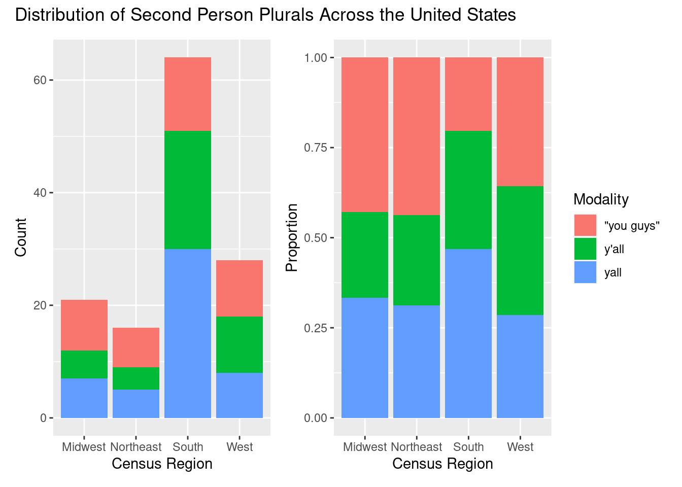
ror_mod_table <-
  xtabs(formula = ~ census_region + search_term, # formula
        data = updated_plurals) # dataset

c2 <- chisq.test(ror_mod_table) # apply the chi-squared test to `ror_mod_table`

c2 # # preview the test results
##
## Pearson's Chi-squared test
##
## data: ror_mod_table
## X-squared = 7.4697, df = 6, p-value = 0.2796#>
#> Pearson's Chi-squared test with Yates' continuity correction
#>
#> data: ror_mod_table
#> X-squared = 101, df = 1, p-value <2e-16
c2$p.value < .05 # confirm p-value below .05## [1] FALSE#> [1] TRUEc2 %>% # statistical result
augment() # view detailed statistical test informationeffects <- effectsize(c2) # evaluate effect size and generate a confidence interval
effects # preview effect size and confidence interval#> Cramer's V | 95% CI
#> -------------------------
#> 0.18 | [0.14, 0.21]
interpret_r(effects$Cramers_v) # interpret the effect size## [1] "small"
## (Rules: funder2019)#> [1] "small"
#> (Rules: funder2019)states_map <- map_data("state") # from ggplot2
p <- ggplot() + geom_polygon(data = states_map, aes(x = long, y = lat, group = group),
fill = "grey", color = "black") + labs(title = "Tweets in the USA", subtitle = "Second Person Plurals")
p + geom_point(data = plurals, aes(x = lng, y = lat, group = 1, color = search_term),
alpha = 1/2, size = 1.5)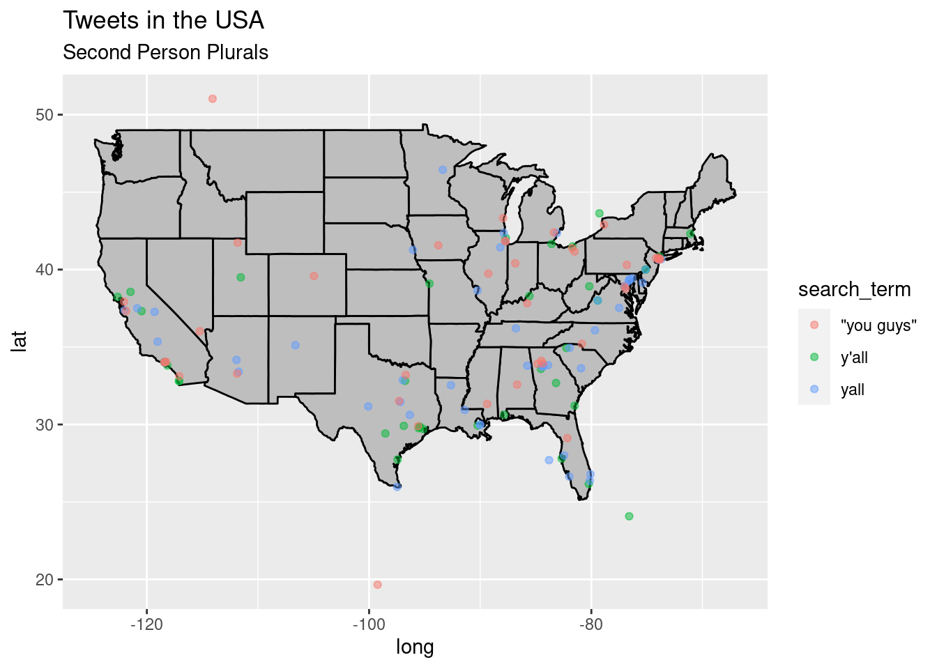
Outdoor Sales
updated_sales %>%
  tabyl(search_term, census_region) %>% # cross-tabulate
  adorn_totals(c("row", "col")) %>% # provide row and column totals
  adorn_percentages("col") %>% # add percentages to the columns
  adorn_pct_formatting(rounding = "half up", digits = 0) %>% # round the digits
  adorn_ns() %>% # add observation number
  adorn_title("combined") %>% # add a header title
  kable(booktabs = TRUE, # pretty table
caption = "Contingency table for `search_term` and `census_region`.") # caption| search_term/census_region | Midwest | Northeast | South | West | Total |
|---|---|---|---|---|---|
| “garage sale” | 50% (3) | 67% (2) | 45% (5) | 43% (6) | 47% (16) |
| “yard sale” | 50% (3) | 33% (1) | 55% (6) | 57% (8) | 53% (18) |
| Total | 100% (6) | 100% (3) | 100% (11) | 100% (14) | 100% (34) |
p1 <-
  updated_sales %>% # dataset
  ggplot(aes(x = census_region, fill = search_term)) + # mappings
  geom_bar() + # geometry
  labs(y = "Count", x = "Census Region") # labels

p2 <-
  updated_sales %>% # dataset
  ggplot(aes(x = census_region, fill = search_term)) + # mappings
  geom_bar(position = "fill") + # geometry, with fill for proportion plot
  labs(y = "Proportion", x = "Census Region", fill = "Modality") # labels

p1 <- p1 + theme(legend.position = "none") # remove legend from left plot

p1 + p2 + plot_annotation("Distribution of Terms for Outdoor Sales Across the US")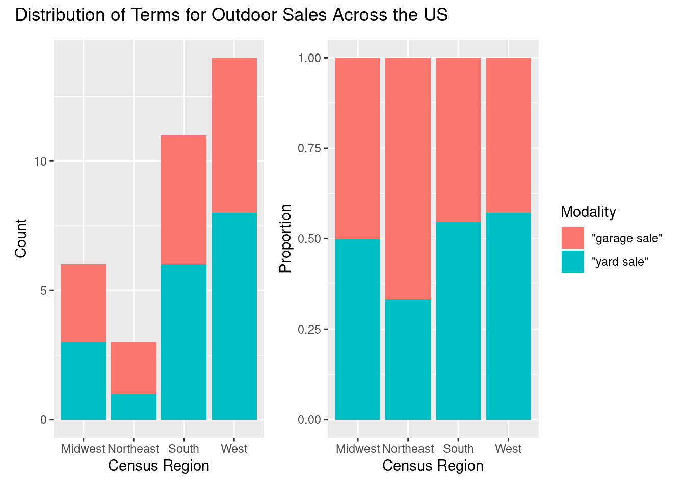
ror_mod_table <-
  xtabs(formula = ~ census_region + search_term, # formula
        data = updated_sales) # dataset

c2 <- chisq.test(ror_mod_table) # apply the chi-squared test to `ror_mod_table`

c2 # # preview the test results
##
## Pearson's Chi-squared test
##
## data: ror_mod_table
## X-squared = 0.59437, df = 3, p-value = 0.8977#>
#> Pearson's Chi-squared test with Yates' continuity correction
#>
#> data: ror_mod_table
#> X-squared = 101, df = 1, p-value <2e-16
c2$p.value < .05 # confirm p-value below .05## [1] FALSE#> [1] TRUEc2 %>% # statistical result
augment() # view detailed statistical test informationeffects <- effectsize(c2) # evaluate effect size and generate a confidence interval
effects # preview effect size and confidence interval#> Cramer's V | 95% CI
#> -------------------------
#> 0.18 | [0.14, 0.21]
interpret_r(effects$Cramers_v) # interpret the effect size## [1] "small"
## (Rules: funder2019)#> [1] "small"
#> (Rules: funder2019)states_map <- map_data("state") # from ggplot2
p <- ggplot() + geom_polygon(data = states_map, aes(x = long, y = lat, group = group),
fill = "grey", color = "black") + labs(title = "Tweets in the USA", subtitle = "Outdoor Sales")
p + geom_point(data = sale, aes(x = lng, y = lat, group = 1, color = search_term),
alpha = 1/2, size = 1.5)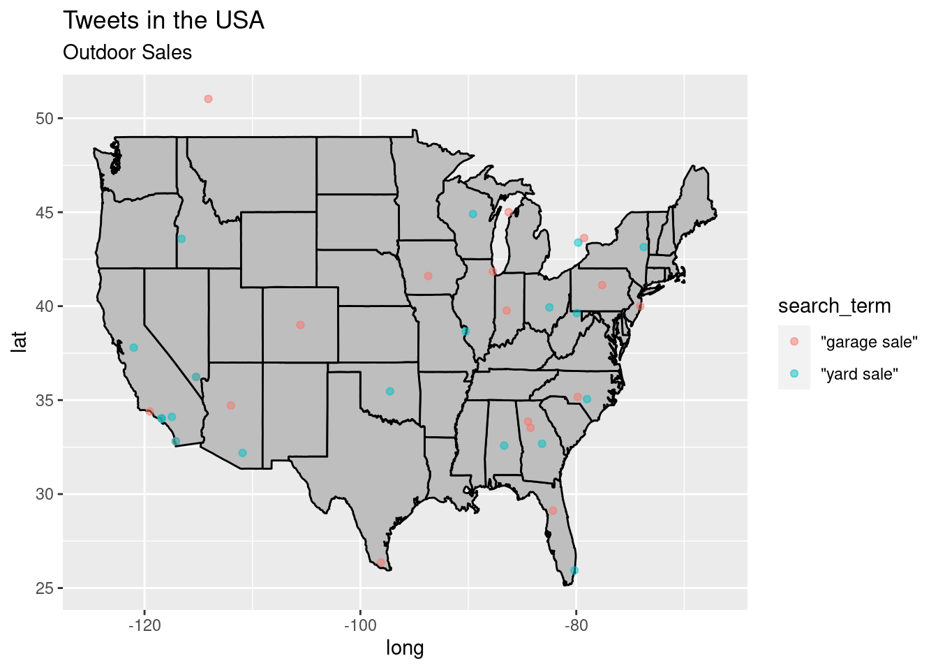
Gym Shoes
updated_shoes %>%
  tabyl(search_term, census_region) %>% # cross-tabulate
  adorn_totals(c("row", "col")) %>% # provide row and column totals
  adorn_percentages("col") %>% # add percentages to the columns
  adorn_pct_formatting(rounding = "half up", digits = 0) %>% # round the digits
  adorn_ns() %>% # add observation number
  adorn_title("combined") %>% # add a header title
  kable(booktabs = TRUE, # pretty table
caption = "Contingency table for `search_term` and `census_region`.") # caption| search_term/census_region | Midwest | Northeast | South | West | Total |
|---|---|---|---|---|---|
| “tennis shoes” | 75% (6) | 0% (0) | 38% (11) | 37% (7) | 34% (24) |
| sneakers | 25% (2) | 100% (15) | 62% (18) | 63% (12) | 66% (47) |
| Total | 100% (8) | 100% (15) | 100% (29) | 100% (19) | 100% (71) |
p1 <-
  updated_shoes %>% # dataset
  ggplot(aes(x = census_region, fill = search_term)) + # mappings
  geom_bar() + # geometry
  labs(y = "Count", x = "Census Region") # labels

p2 <-
  updated_shoes %>% # dataset
  ggplot(aes(x = census_region, fill = search_term)) + # mappings
  geom_bar(position = "fill") + # geometry, with fill for proportion plot
  labs(y = "Proportion", x = "Census Region", fill = "Modality") # labels

p1 <- p1 + theme(legend.position = "none") # remove legend from left plot

p1 + p2 + plot_annotation("Distribution of Terms for Gym Shoes Across the United States")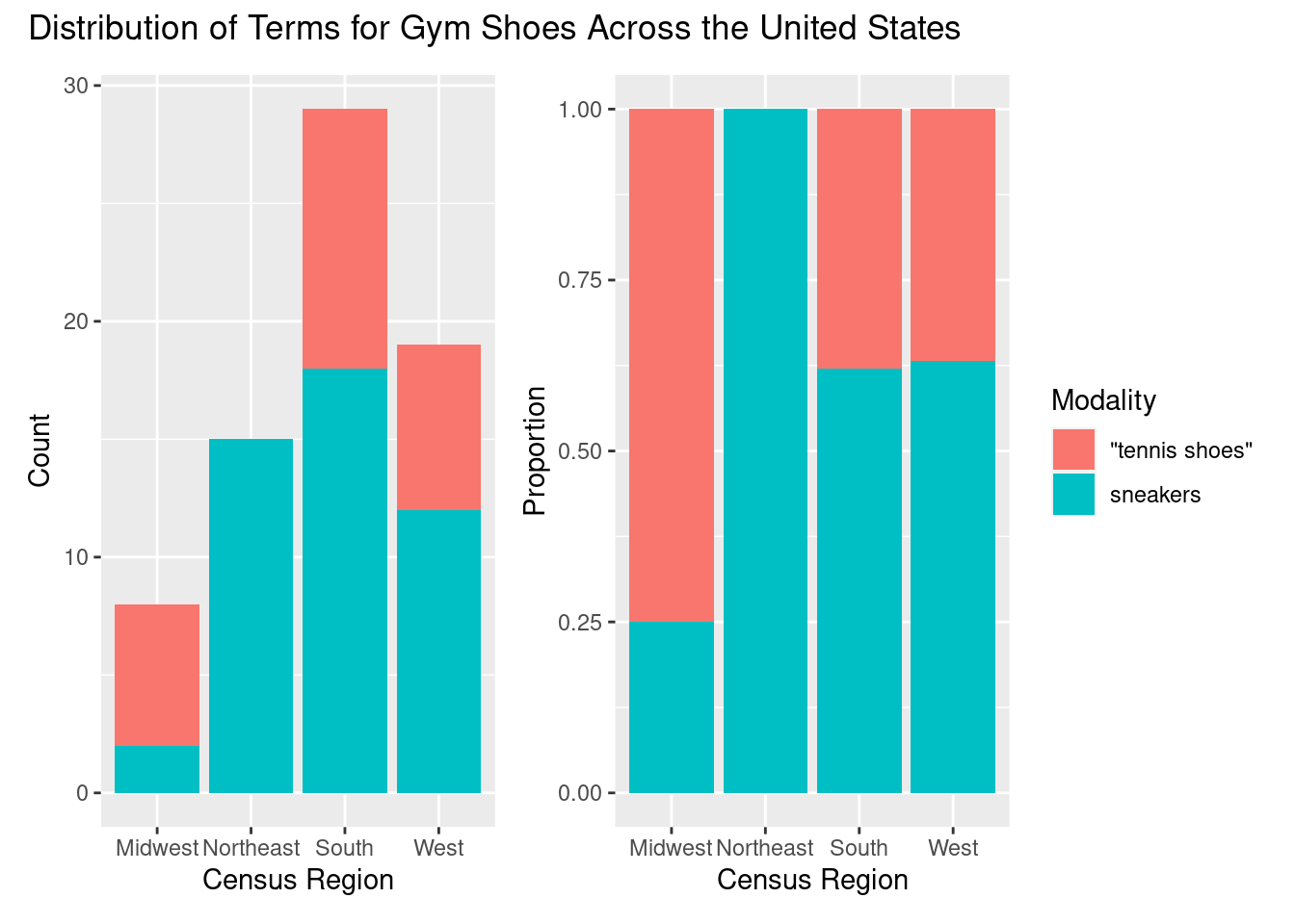
ror_mod_table <-
  xtabs(formula = ~ census_region + search_term, # formula
        data = updated_shoes) # dataset

c2 <- chisq.test(ror_mod_table) # apply the chi-squared test to `ror_mod_table`
## Warning in stats::chisq.test(x, y, ...): Chi-squared approximation may be incorrectc2 # # preview the test results##
## Pearson's Chi-squared test
##
## data: ror_mod_table
## X-squared = 14.027, df = 3, p-value = 0.002869#>
#> Pearson's Chi-squared test with Yates' continuity correction
#>
#> data: ror_mod_table
#> X-squared = 101, df = 1, p-value <2e-16
c2$p.value < .05 # confirm p-value below .05## [1] TRUE#> [1] TRUEc2 %>% # statistical result
augment() # view detailed statistical test informationeffects <- effectsize(c2) # evaluate effect size and generate a confidence interval
effects # preview effect size and confidence interval#> Cramer's V | 95% CI
#> -------------------------
#> 0.18 | [0.14, 0.21]
interpret_r(effects$Cramers_v) # interpret the effect size## [1] "very large"
## (Rules: funder2019)#> [1] "small"
#> (Rules: funder2019)states_map <- map_data("state") # from ggplot2
p <- ggplot() + geom_polygon(data = states_map, aes(x = long, y = lat, group = group),
fill = "grey", color = "black") + labs(title = "Tweets in the USA", subtitle = "Shoes")
p + geom_point(data = shoes, aes(x = lng, y = lat, group = 1, color = search_term),
alpha = 1/2, size = 1.5)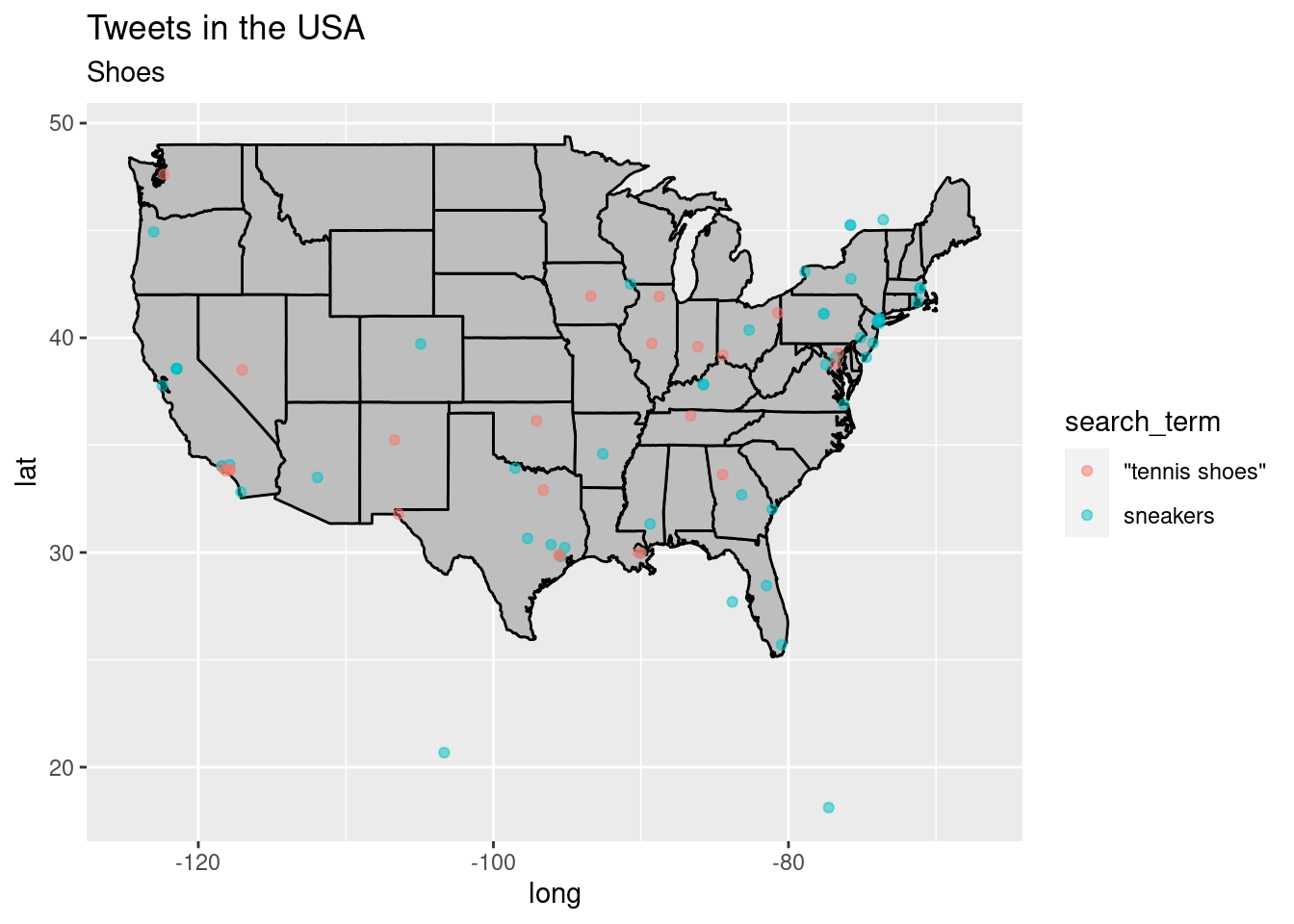
Soft Drinks
updated_tonix %>%
  tabyl(search_term, census_region) %>% # cross-tabulate
  adorn_totals(c("row", "col")) %>% # provide row and column totals
  adorn_percentages("col") %>% # add percentages to the columns
  adorn_pct_formatting(rounding = "half up", digits = 0) %>% # round the digits
  adorn_ns() %>% # add observation number
  adorn_title("combined") %>% # add a header title
  kable(booktabs = TRUE, # pretty table
caption = "Contingency table for `search_term` and `census_region`.") # caption| search_term/census_region | Midwest | Northeast | South | West | Total |
|---|---|---|---|---|---|
| coke | 49% (22) | 43% (16) | 37% (36) | 27% (17) | 37% (91) |
| pop | 24% (11) | 19% (7) | 30% (29) | 27% (17) | 26% (64) |
| soda | 27% (12) | 38% (14) | 34% (33) | 46% (29) | 36% (88) |
| Total | 100% (45) | 100% (37) | 100% (98) | 100% (63) | 100% (243) |
p1 <-
  updated_tonix %>% # dataset
  ggplot(aes(x = census_region, fill = search_term)) + # mappings
  geom_bar() + # geometry
  labs(y = "Count", x = "Census Region") # labels

p2 <-
  updated_tonix %>% # dataset
  ggplot(aes(x = census_region, fill = search_term)) + # mappings
  geom_bar(position = "fill") + # geometry, with fill for proportion plot
  labs(y = "Proportion", x = "Census Region", fill = "Modality") # labels

p1 <- p1 + theme(legend.position = "none") # remove legend from left plot

p1 + p2 + plot_annotation("Distribution of Terms for Soft Drinks Across the US")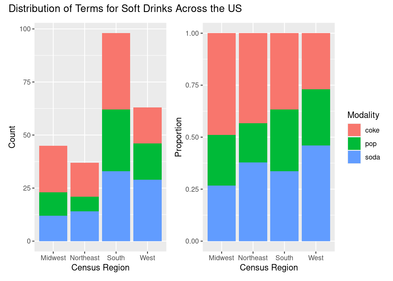
ror_mod_table <-
  xtabs(formula = ~ census_region + search_term, # formula
        data = updated_tonix) # dataset

c2 <- chisq.test(ror_mod_table) # apply the chi-squared test to `ror_mod_table`

c2 # # preview the test results
##
## Pearson's Chi-squared test
##
## data: ror_mod_table
## X-squared = 8.0096, df = 6, p-value = 0.2374#>
#> Pearson's Chi-squared test with Yates' continuity correction
#>
#> data: ror_mod_table
#> X-squared = 101, df = 1, p-value <2e-16
c2$p.value < .05 # confirm p-value below .05## [1] FALSE#> [1] TRUEc2 %>% # statistical result
augment() # view detailed statistical test informationeffects <- effectsize(c2) # evaluate effect size and generate a confidence interval
effects # preview effect size and confidence interval#> Cramer's V | 95% CI
#> -------------------------
#> 0.18 | [0.14, 0.21]
interpret_r(effects$Cramers_v) # interpret the effect size## [1] "small"
## (Rules: funder2019)#> [1] "small"
#> (Rules: funder2019)states_map <- map_data("state") # from ggplot2
p <- ggplot() + geom_polygon(data = states_map, aes(x = long, y = lat, group = group),
fill = "grey", color = "black") + labs(title = "Tweets in the USA", subtitle = "Soft Drinks")
p + geom_point(data = tonix, aes(x = lng, y = lat, group = 1, color = search_term),
alpha = 1/2, size = 1.5)## Warning: Removed 5724 rows containing missing values (geom_point).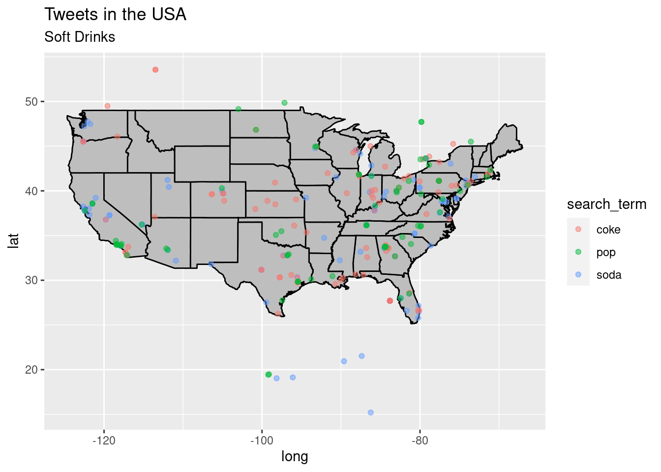
Major Roads
updated_roads %>%
  tabyl(search_term, census_region) %>% # cross-tabulate
  adorn_totals(c("row", "col")) %>% # provide row and column totals
  adorn_percentages("col") %>% # add percentages to the columns
  adorn_pct_formatting(rounding = "half up", digits = 0) %>% # round the digits
  adorn_ns() %>% # add observation number
  adorn_title("combined") %>% # add a header title
  kable(booktabs = TRUE, # pretty table
caption = "Contingency table for `search_term` and `census_region`.") # caption| search_term/census_region | Midwest | Northeast | South | West | Total |
|---|---|---|---|---|---|
| freeway | 26% (6) | 18% (4) | 61% (39) | 61% (60) | 52% (109) |
| highway | 74% (17) | 82% (18) | 39% (25) | 39% (39) | 48% (99) |
| Total | 100% (23) | 100% (22) | 100% (64) | 100% (99) | 100% (208) |
p1 <-
  updated_roads %>% # dataset
  ggplot(aes(x = census_region, fill = search_term)) + # mappings
  geom_bar() + # geometry
  labs(y = "Count", x = "Census Region") # labels

p2 <-
  updated_roads %>% # dataset
  ggplot(aes(x = census_region, fill = search_term)) + # mappings
  geom_bar(position = "fill") + # geometry, with fill for proportion plot
  labs(y = "Proportion", x = "Census Region", fill = "Modality") # labels

p1 <- p1 + theme(legend.position = "none") # remove legend from left plot

p1 + p2 + plot_annotation("Distribution of Terms for Major Roads Across the US")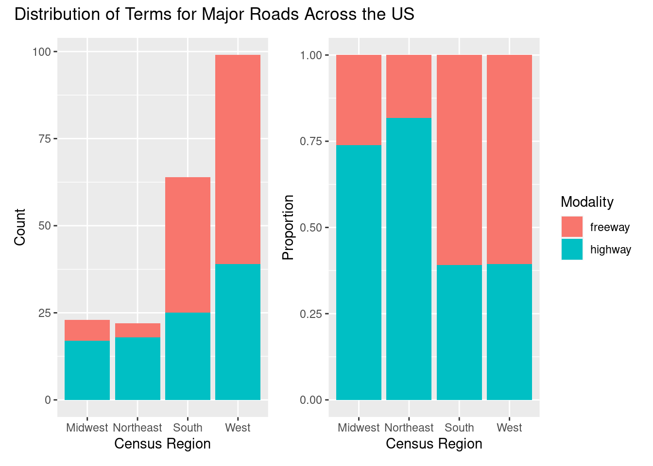
ror_mod_table <-
  xtabs(formula = ~ census_region + search_term, # formula
        data = updated_roads) # dataset

c2 <- chisq.test(ror_mod_table) # apply the chi-squared test to `ror_mod_table`

c2 # # preview the test results
##
## Pearson's Chi-squared test
##
## data: ror_mod_table
## X-squared = 21.255, df = 3, p-value = 9.317e-05#>
#> Pearson's Chi-squared test with Yates' continuity correction
#>
#> data: ror_mod_table
#> X-squared = 101, df = 1, p-value <2e-16
c2$p.value < .05 # confirm p-value below .05## [1] TRUE#> [1] TRUEc2 %>% # statistical result
augment() # view detailed statistical test informationeffects <- effectsize(c2) # evaluate effect size and generate a confidence interval
effects # preview effect size and confidence interval#> Cramer's V | 95% CI
#> -------------------------
#> 0.18 | [0.14, 0.21]
interpret_r(effects$Cramers_v) # interpret the effect size## [1] "large"
## (Rules: funder2019)#> [1] "small"
#> (Rules: funder2019)states_map <- map_data("state") # from ggplot2
p <- ggplot() + geom_polygon(data = states_map, aes(x = long, y = lat, group = group),
fill = "grey", color = "black") + labs(title = "Tweets in the USA", subtitle = "Major Roads")
p + geom_point(data = roads, aes(x = lng, y = lat, group = 1, color = search_term),
alpha = 1/2, size = 1.5)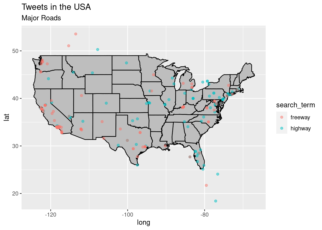
Finalize
Log
This code should produce bar charts, contingency tables, maps, and information about each chi-squaured test conducted.
References
Vaux, Bert. “Harvard Dialect Survey.” Harvard Dialect Survey, 2003, http://dialect.redlog.net.